How to build your own appraisal form in Excel (a primer with pics)

[George Hatch]

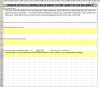
Okay - next up we'll do some copy/paste and some transfers

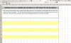
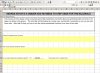
right click the text field, hit "copy", then go to line 6 and use the paste icon on the toolbar to paste and hit enter. Then delete the text and delete the border (using the border command or by using the eraser on the line formatting box) , copy that field and use the arrow key and the paste command to add more text fields to your page. You can resize the length of each field individually or highlight a bunch of them and resize them all at the same time and to the same size.

If/when you exceed your print margins that entire field will be printed on the next page, so resizing these fields is one way to make these pages look uniform. I've colored these copied text fields yellow so you can see them

 

[George Hatch]

Now go back and add some "form" text. As I say, I use a smaller font for the form verbiage so the readers can see which is which.

 

[George Hatch]

Merge q1 and r1, and use that field for your file number, and then go down to the lower right hand corner of whatever your print range is and (for now) add a "1" for your page number. It should look like this

 

[George Hatch]

Now copy your entire page and paste it into sheet2 of your file (next page). Obviously it will look exactly the same until you change it.

Now I'll show you transfers. Delete the file number and page number on sheet2. Then go into the file number cell on sheet2, and type "=" and go to the corresponding field on sheet1 and hit enter. The *field* will show the same as on sheet1, but *equation* in the field section on sheet2 will now read "=sheet1!Q1" or whatever cell on sheet1 you put that file number in. Those equations don't show in your printout unless you format them to show - which we're not going to do.

Now go to the page number cell in the lower right hand corner and type in "=1+" and go to that cell on sheet1 and hit enter. The *field* will show a "2" but the *equation* line up on top will show "=1+Sheet1!Q22"

So now really, aside from learning how to write the math equations (also pretty simple) that's about it for form design. Those are all the commands and processes you need to use. You can use that transfer process to copy addresses or parcel numbers of GLA numbers from one page to another throughout the report. You can add borders and form columns and lines and such. You can add checkboxes if you're into those (Personally, I mostly avoid them) . You can format cells to show dates or currency or numbers or text or percentages and such. And obviously you can do the math because, after all, these are spreadsheets.

 

[Renee Healion]

Thanks, George. This was generous of you.

For non GSE stuff, I mostly use the AI form suite, or write narrative and add in snips of excel grids or the AI grid as exhibits. But this could be a good way to offer a service I have been thinking about which comes up periodically.

 

[George Hatch]

Thx for taking the time to work your way through it. I think you've got it.

For your text boxes you can hold the control key and highlight all of them at the same time, and hit the "align left" button in your toolbar. The text fields for the address can all be transferred anywhere else in the form so if you make the change in the source field (the one where you would initially add the info) it will get copied everywhere you tell it to copy. However, when the contents of a field that was formatted to show as a number gets transferred only the number itself goes, not the formatting; so you'll have to format the new cell.

 

[George Hatch]

Now for "special" formatting.

Let's say you wanted to your lot area to display like this: "10,000 sf", or your file number to show like "File# 21" or your page number to show "Pg 1" - here's the process for that

right click the field
"format cells" and the dialog box will show up,
click "number" and scroll down to the bottom of your list of choices (which include date, currency, text, percentage, fraction, etc) to "custom"
The first choice is a "0" - use that one for numbers you don't want to display with the thousands separator. Use the 3rd choice when you do want the number to show with a thousands separator, like 1,000 vs 1000.

For now pick the 3rd one which shows x,xx0 and replace the 0 with quotation marks and whatever text you want to display. Don't forget the space if you want there to be a space between the number and the text, so it looks like this:
x,xx" sf"

then when you go to use that field in your form and you enter 100 it will display as:
100 sf

Same thing for adding a prefix: formatting
"File No. "x
will display as
File No. 102
when you put that 102 into the field

 

[George Hatch]

Now for a simple adjustment grid. Start with a fresh page, and highlight the entire columns from A to K (that will be 11 columns). Widen the width from 5.00 to 10.00. Then format A thru E like this:

 

[George Hatch]

We've got some merging, some borders, some form vs text font sizing, some number and prefix formatting and an underline text for the adjustments number.

Now we're going to add the math. Go into cell E5 and enter this formula:\
=(B5-D5)*C5

Basically, you're telling the spreadsheet to subject the lot area for Sale #1 from the subject's lot area and then multiply that result times the adjustment factor in C5. Since you already had numbers for lot area for the subject and S#1 the spreadsheet will already have calculated that adjustment at $1000. If you change any of those numbers the spreadsheet will do the calculation automatically. Now to anchor the subject columns in the equation so it will work no matter where the comparable line is in the worsheet just modify the subject references by adding a $ sign in front of the column and line references in that equation so it looks like this:

=($B$5-D5)*$C$5

Now only the comparables reference will float. You can other copy/paste that equation into the cell below or simply rewrite the equation for that line:

=($B$6-D6)*$C$6

Now the last thing for Sale #1 is to do the addition:

Highlight E5 to E8 with your mouse and hit the autosum button on your toolbar - it's the one that looks like the backwards 3, or write the equation
=sum(e5:E7)

Then add your adjustments to your sale price in E9 to get your adjusted value indicator. Go to E9:
=E3+E8

By this time it should look like this:

 

[George Hatch]

Obviously, it takes a lot longer to read my instructions on doing this than to do it. After about the 3rd or 4th time it'll go as fast as you can decide what it is you want to do.

Now, copy/paste the "Sale #1 column into the other columns to the right, however many you want to add, and then rename them in the header line. I'm just going to do 4 of them for now. You can test everything to see if it's working as intended by changing the numbers on each comparable.